Linear Regression

Linear Regression

features of customer: \(x = (x_0, x_1, x2, ..., x_d)\) ,

approximate the desired credit limit with a weighted sum:

\[y \approx \sum_{i=0}^{d} w_i X_i = \begin{bmatrix} w_0 \\ w_1 \\ \cdots \\ w_d \end{bmatrix} \cdot \begin{bmatrix} x_0 \ x_1 \ \cdots \ x_d \end{bmatrix}\]

linear regression hypothesis: \(h(x) = w^T x\)

\[y = (x_1) \in \mathbb{R} \ \ \ \ \ \ y = (x_1, x_2) \in \mathbb{R}^2\]

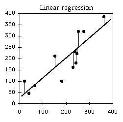
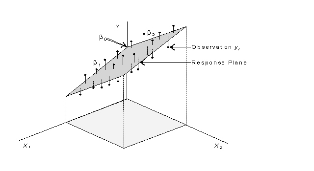
Find lines / hyperplanes with small residuals

Error Measure

squared error : \(err(\hat{y}, y) = ( \hat{y} - y )^2\)

in-sample:

\[\begin{align} & E_{in}(h) = \frac{1}{N} \sum_{n=1}^{N} \left( h(x_n) - y_n \right)^2 \ \ \rightarrow \ \ & E_{in}(w) = \frac{1}{N} \sum_{n=1}^{N} \left( w^Tx_n - y_n \right)^2 \end{align}\]

out-of-sample:

\[E_{out}(w) = \varepsilon_{(x,y) \sim P} ( w^T x - y )^2\]

Find minimum \(E_{in}\)

\[E_{in}(w) = \frac{1}{N} \sum_{n=1}^{N} \left( w^Tx_n - y_n \right)^2 = \frac{1}{N} \sum_{n=1}^{N} \left( x_n^T \underline{w} - y_n \right)^2 \\ =\frac{1}{N} \begin{Vmatrix} x_1^T w & - & y_1 \\ x_2^T w & - & y_2 \\ ... & & \\ x_N^T w & - & y_N \\ \end{Vmatrix} ^2\] \[=\frac{1}{N} \begin{Vmatrix} \begin{bmatrix} x_1^T \\ x_2^T \\ ... \\ x_N^T \\ \end{bmatrix} w - \begin{bmatrix} y_1 \\ y_2 \\ ... \\ y_N \end{bmatrix} \end{Vmatrix}^2 \\ =\frac{1}{N} \begin{Vmatrix} \\ \underline{\underline{X}} \underline{w} - \underline{Y} \\ \end{Vmatrix}^2\]

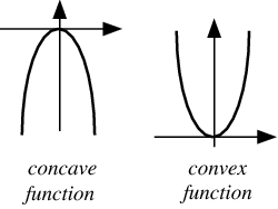
this is a convex function. So, find \(w_{LIN}\) such that \(\triangledown E_{in}(w_{LIN}) = 0\)

\[min_w E_{in}(w)=\frac{1}{N} \begin{Vmatrix} X w - Y \end{Vmatrix}^2 = \frac{1}{N} ( w^T X^T X w - 2 w^T X^T y + y^T y )\]

let array ‘A’ = \(X^T \ X\), vector ‘b’ = \(X^T \ y\), constant ‘c’ = \(y^T \ y\). The equation can be changed to:

\[\begin{align} E_{in}(w) & = \frac{1}{N} ( w^T A w - 2 w^T b + c ) \\ \nabla E_{in}(w) & = \frac{1}{N} ( 2 A w - 2 b ) \\ \nabla E_{in}(w) & = \frac{2}{N} ( X^T X w - X^T y ) \\ \end{align}\]

for invertible \(X^T X : w_{LIN} = ( X^T X )^{-1} X^T y = X^{\dagger} y\)

pseudo-inverse : \(X^{\dagger} = ( X^T X )^{-1} X^T\)

practical suggestion

use well-implemented \(\dagger\) routine

Summary of Linear Regression Algorithm

1. from Data, construct input matrix X ( Nx(d+1) columns ) and output vector y ( Nx1 columns )

   \[X = \begin{Vmatrix} - - x_1 - - \\ - - x_2 - - \\ - - \cdots - - \\ - - x_N - - \\ \end{Vmatrix} \ \ \ \ y = \begin{pmatrix} y_1 \\ y_2 \\ \cdots \\ y_N \\ \end{pmatrix}\]
2. calculate pseudo-inverse \(X^\dagger\) : (d+1)xN columns
3. return \(W_{LIN} = X^\dagger y\) : (d+1)x1 columns

Coding example in R

data from this artical, here is the r code

---

avg of E_in = noise_level x \(( 1 - \frac{d+1}{N} )\)

call \(XX^{\dagger}\) the hat matrix H, because it puts ^ on y

The learning Curve

expected generalization error: \(\frac{2(d+1)}{N}\)